Module 4 - Config Creator
Introduction to the Config Creator
The OptaSense Config Creator has been developed to allow system configs to be created with ease. All new System configs should be created using this utility. If the config has not been created properly using this utility, it will invariably result in the OptaSense software failing to launch
Note: Use of Config Creator requires a valid licence.
Installing the Config Creator
- To start the process of installing the creator, run the executable. The Config Creator installation screen will appear (Figure 1).
Contact OptaSense for the downloadable link, if required.
Figure 1: Config Creator Setup Installation Screen
- Click Next and then Install the program to the default directory (Figure 2). If necessary, the installation destination can be changed.
Figure 2: Select Destination Folder for Config Creator
- The creator will now install. Select Finish when prompted (Figure 3).
Figure 3: Finishing the installation
Using the Config Creator
To run the config creator, launch it from the Windows Start menu. Two options will be offered: "New System" and "Load from Existing Config" (Figure 4).
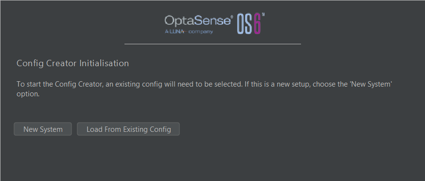
Figure 4: Config Creator Launch Screen
To create a new config, select the New System button. The next window asks the user to set the OPS's required for the system (Figure 5).
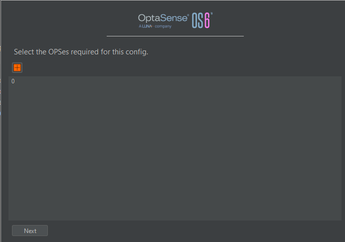
Figure 5: Selecting number of OPS's
The second option available at the creator launch screen is an option to open an existing config folder. It is possible to modify the current settings of a config, which can then be saved and exported to be used with the OptaSense software. When opening an existing config, the same screens and tabs that are available when creating the config are available for editing the config.
System Sepecfication Editor
The first item to create is the ‘System Specification’ file. From the main menu (Figure 6), select System Specification Editor.

Figure 6: Giving the system a specification

Figure 7: System Speciification Editor
Once this display is open, refer to ‘Module 12 – Adding New PU(s) To the System’, for adding new PUs and its processing/interfaces.
Once the required PUs have been added to the specification editor, the Operator will need to ‘Apply Changes’ which will store the updated system specification in the config creator.
Georeferenced Imagery Selection
Prior to creating the config, the user should have acquired the imagery to follow the asset route. Imagery is not necessary for creating a fibre route but significantly improves visual understanding of the system. The required standards for imagery are:
- Images to be GEOTIFF format using EPSG 4236 (WGS-84) with any null-imagery pixels to be set to digital black (0,0,0).
- OptaSense normally advises a maximum resolution of 1m sized pixels and an overview image resolution of 15m pixels.
It is also possible to use static imagery and apply manual geo-referencing but this can lead to issues if the aspect ratio of the images is not correct.
To access the imagery section, select Imagery from the Configure menu.
Imagery Pre-Processing
On the right-hand side of the Imagery window, select Import GeoTIFF Folder and navigate to the required folder. Select OK to process the imagery. Once finished, the window will say Processing Complete.
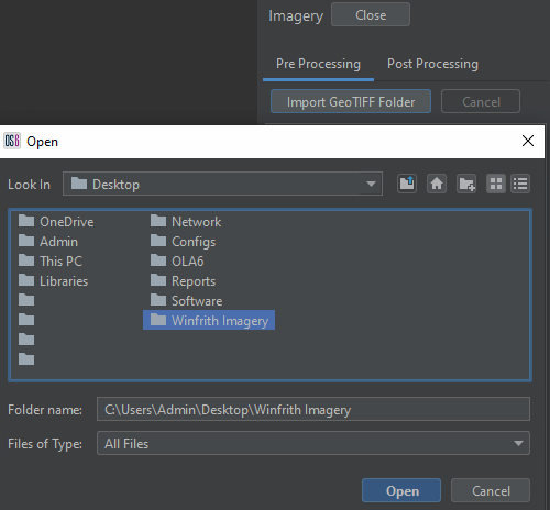

Figure 13: Adding GeoTIFF Files
If there are further images to pre-process, repeat the last paragraph and when asked to add layer or to overwrite the existing images, choose add layer (Figure 14).

Figure 14: Adding Another GeoTIFF Layer
Post Processing
The post processing window enables the user to add the pre-possessed imagery or add a static image and manually geo-reference it.
Using Preprocessed GeoTIFF's
To add the pre-processed image(s), select the globe icon (Figure 15). The layer can be re-named appropriately or left as default. Check the Add Layer box to make the imagery visible and select OK.
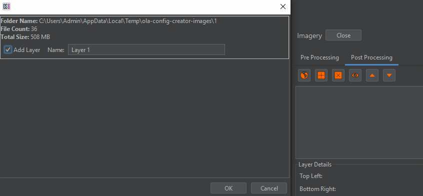
Figure 15: Making Layer Visible
The screen will refresh, and the imagery will be displayed (Figure 16).

Figure 16: Imagery Visible
If multiple layers were added but the imagery looks to be missing sections, the layer order may need changing. To do this, select 1 of the layers and use the up and down arrows to reorder (Figure 17).
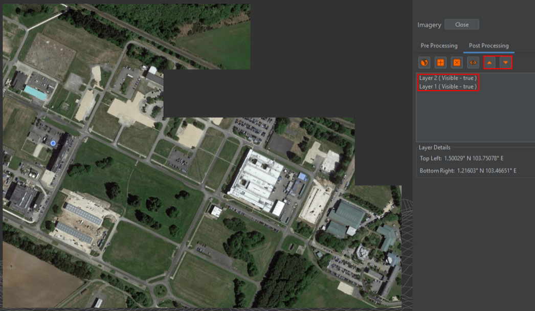
Figure 17: Unordered Layers
Manually Georeferencing Static Images
To import a static image, select the square with a cross icon and navigate to the required image (Figure 18). Name the layer appropriately and select next.
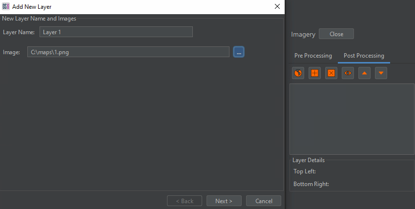
Figure 18: Selecting Static Image
The aim of this step is to manually geo-reference an image using latitude / longitude (LAT / LONG) co-ordinates. To do this, identify a point in the top-left and bottom-right corner of the image that will act as the reference points. Select the button under the Top-Left Calibration Point section (Figure 19). Select the previously identified point in the top-left of the image – the location will be marked by a red cross on the image - and input the LAT/LONG co-ordinates for this position in the Set Position box that appears. Select OK to confirm the position. Repeat the process for the point identified in the bottom-right of the image. Note: the diagonal arrow buttons can be used to zoom into the top-left and bottom-right regions of the image to assist in selecting the calibration position. Select Finish to complete geo-referencing the static imagery.
This process can be repeated for multiple static images.
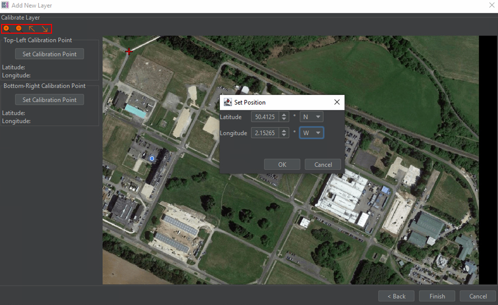
Figure 19: Geo-referencing Static Imagery
Map Positioning
Map positioning enables the user to set zoom levels. To access this section, select Map Positioning from the Configure menu.
Use the mouse scroll wheel to zoom in to the desired maximum zoom level. Click the arrow icon next to the Zoom In Limit box (Figure 20). Zoom out to the desired minimum zoom level and click the arrow to select this as the Zoom Out Limit.
Note: Setting these limits will impact how far a user can zoom in and out when in OS6 but will not limit zoom levels within the Config Creator.
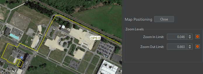
Figure 20: Setting Zoom in / out Positions on Map Display
Fibre Configuration
The fibre route section enables the user to create the systems fibre route(s). This is essentially the route that represents the path of the sensing fibre on the map.
To access the Fibre Route section, select Fibre Route from the Configure menu. The fibre route can be built from scratch or imported from file into the creator.
Building New Fibre Route
To build from scratch, use the three drawing buttons highlighted in red in Figure 21.
- Left button: add a point
- Middle button: delete a point
- Right button: move apoint.
The first co-ordinate point (node) added is the starting point. Two nodes are required to draw the first line.
There are two ways to delete nodes:
- Select the delete button highlighted in red below. Now click on the required node to delete it.
- Right click on the required node. Select the Delete button highlighted in blue.
It's advisable to save changes every couple of actions. This is to enable the user to revert to a known state by clicking Undo if a mistake has been made.
The options highlighted by the green box on Figure 21 enable the user to visually turn on / off additional fibre information.
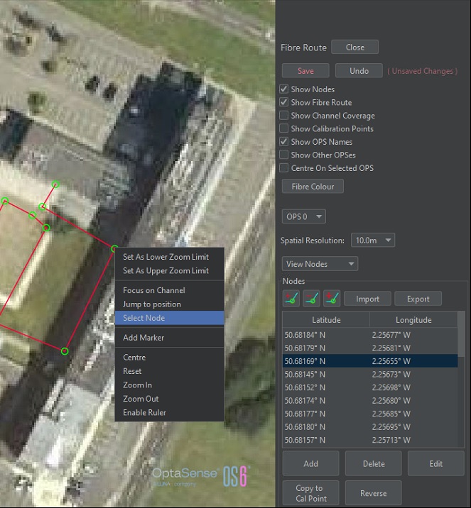
Figure 21: Fibre Route Creation
Importing Existing Fibre Route
An alternative to manually drawing a fibre route is to import a list of known co-ordinates. To ensure that the co-ordinates can be imported the following checks can be carried out.
- The route data must be in LAT/LONG or UTM format and arranged in two columns.
- The latitude/easting co-ordinate should be in the first column
- The file should be save as CSV (Comma Separated Values).
Fibre routes can be prepared according to this specification in a variety of programmes, such as Excel and Notepad++ (Figure 22).
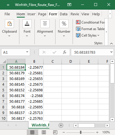
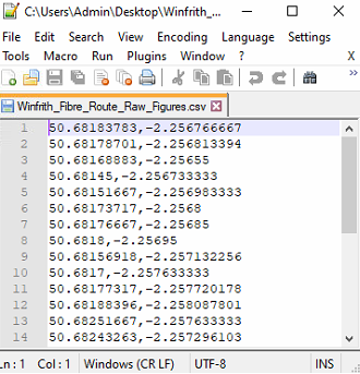
Figure 22: (Left) Using Excel to compile. (Right) Using Notepad++ to compile
To import a fibre route, select the Import button and choose the required file (Figure 23). Choose the required co-ordinate system, LAT/LONG or UTM (Universal Transverse Mercator). Increasing the Thinning Factor enables the user to reduce the number of nodes that will be imported. This is useful for files that contain an excessive and unnecessary number of nodes. Select OK to complete the import.
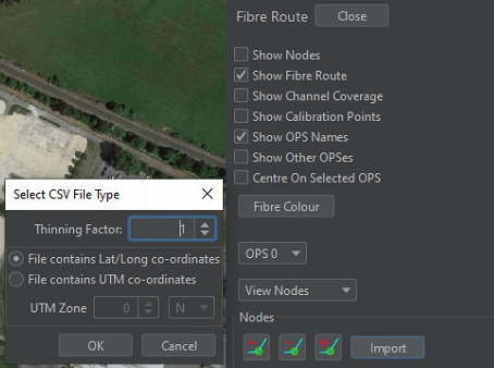
Figure 23: Importing Fibre Route
Calibration
Calibration (cal) points provide information about the optical distance between different locations, as well as a unique name and geographical reference for its placement. These are required because fibre routes often break out into junction boxes, contain optical coils and deviate from the path of the monitored asset so that the optical path length exceeds the length of the monitored asset. Physically obtaining cal points essentially involves generating a signal at a known location and identifying the equivalent optical distance on the system – the process is covered in more detail in Module 10 - Calibration and Geo-referencing Procedure. If the cal points are already known then they can be added into the fibre route using the following procedure.
In the fibre route panel, switch from View Nodes to View Cal Points by selecting the option from the drop-down box (Figure 24).
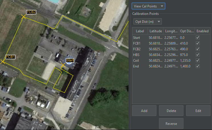
Figure 24: View Cal Point
There are several ways to add a cal point:
- Select Add from the Calibration Points section.
- Select a node from the Node list and select Copy to Cal
The first option will produce the Add Calibration Point box (Figure 25). The latter option requires selection of the new point in the Cal Point table and then selecting Edit.
Provide the cal point with a useful Label, GPS co-ordinates and appropriate Optical Distance information. Cal points can also be specified in Channels if preferred by switching the Opt Dist (m) box to Channels.
Confirm the point information is correct and select OK to add it.
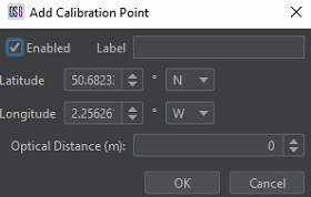
Figure 25: Confirm Cal Point Info is Correct
If a cal point is not currently in use or the system has identified an issue then the cal point will be highlighted in red in the table. This can happen if a cal point is specified too far away from the fibre route or if the requirements of the cal point are physically not possible i.e. the optical path length is shorter than the physical path length.
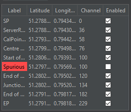
Figure 26: Erroneous Cal point
With cal points entered, the user can verify their accuracy by enabling Show Channel Coverage (Figure 27. Each channel is represented by an open circle of diameter equal to the spatial resolution currently being used (e.g. 5m, 10m etc). If a coil of fibre is present then the optical channels will overlap on top of each other. If there's a significant gap between the circles then this indicates a problem with the node routing or that a cal point is incorrect. For linear segments of fibre, the channel circles should barely overlap.
Note: Optical coils generally require two cal points at the same location to allow the route to be properly calibrated
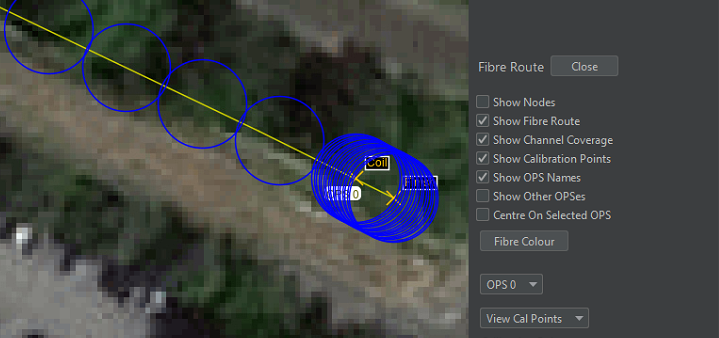
Figure 27: Channel coverage showing an fibre coil and linearly spaced channels
Custom Routes
Paths
Paths can be created on the Map screen to highlight features like roads, tracks, rivers and other geographical markers.
To begin creating a path, select Custom Routes from the Configure tab.
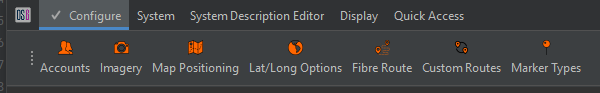
Figure 28: Custom Routes Location
Clicking 'Add' will load the add new custom route dialogue box up an Input box and prompt for a new for the new path. Ensure that the Route Type is set to "Path", enter a path name and click OK. The colour can be changed before selecting OK if desired.
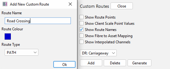
Figure 29: Path creation from custom routes
To start drawing a path, select the Add Route Nodes button in the custom routes dialogue and click on the map display where the first point is positioned. Select a second point, to which a line will be drawn. Additional points can be added between two existing nodes by creating a node close to the line between the two nodes. To remove a point, slect the Remove Route Nodes button and click on the required point to delete it. Selecting the Move Route Nodes button allows existing nodes to be manipulated into a different position. Once the path is drawn, either add more custom routes as required or press Close. Pressing Close will open a Save changes prompt where changes can be saved or ignored. If adding multiple routes it is advisable to save changes regularly.

Figure 30: Path on the map display
Asset Route
Asset route mapping allows the operators to create custom routes that can be used within detectors to address the differences between the fibre route and the physcial asset – for instance, the effect of optical coils. Asset routes make use of a 'Fibre to Asset Mapping' algorithm to enable monitoring of an asset in relation to the monitored fibre. Notable examples where this would prove useful would be road and rail assets.
Only the Road Detector currently makes use of Asset Routes.
To create an Asset Route, select configure custom routes from the toolbar and add a new route. Give the Asset Route a name and ensure that Asset Route is selected in the drop-down menu (Figure 81). An Asset Route will always be mapped to Fibre Channels.
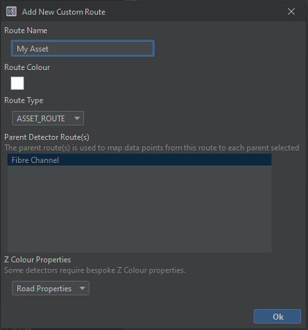
Figure 31: Asset Route Creation
Select OK to create the route. It is then possible to add/remove and move Asset points on the map from the asset dialogue. As shown in Figure 32, once an asset route has been created, if the Show Fibre to Asset checkbox is selected, the interpolated channel mapping to each asset channel is visible (denoted by the short blue lines).
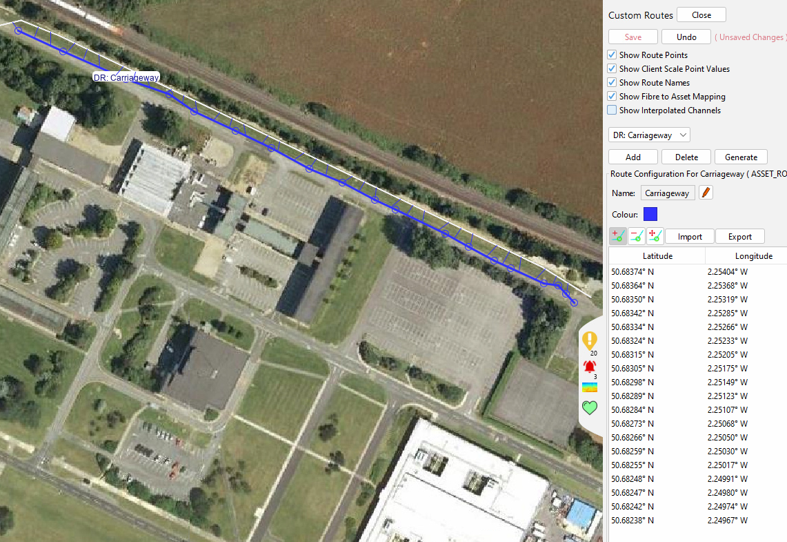
Figure 32: Asset Route showing mapping to OPS channels
Assets can be grouped into Detector Routes which consists of Fibre and Asset Routes
Client Scale
The client scale is used to plot a series of reference points along Detector Routes – most commonly K-points along pipelines. A client scale allows alerts to be output using a scale they are more familiar with. The client scale can also be displayed on the x-acis of the ‘Waterfall’ display. When using a client scale on the waterfall display the x-axis will always increase from left-to-right; The fibre channels will automatically be flipped if the scale runs in the reverse order to the fibre channels. While a Client Scale can span multiple OPS, the waterfall display will only display the section that is relevant to the currently selected OPS.
Utilising the 'Fibre to Asset Mapping' mechanism means it is possible to create client scales that follow an asset (e.g. a pipeline) rather than the fibre route. This allows unnecessary fibre channels to be removed from the fibre route when displayed on the waterfall (for instance, optical coils or fibre around a block valve station). Multiple Client scales can be created to allow a waterfall to show just the relevant channels for different routes.
Adding a New Client Scale
To add a client scale, open the custom routes dialogue and choose Add. Provide a name for the scale, colour and select Client Scale from the drop-down menu. The table at the bottom allows the selection of different parent routes so that client scales can be mapped to Assets Routes instead of OPS.
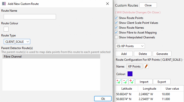
Figure 33: Client Scale
Select OK to create the Client Scale. It is then possible to add, remove and move client scale points on the map. Unique User values must be assigned to each point, and these will be interpolated between pairs of points along the defined route. Checking the 'Show Interpolated Channels' flag will show each client scale channel as a circle along the route. Checking the 'Show Fibre to Asset Mapping' flag will draw lines showing the mapping of each client scale channel to the parent route channel (denoted by the short blue lines in Figure 34).
If co-ordinates are available in the appropriate CSV format, then these can be imported via the import button. Similarly, a defined client scale can be exported.
When creating a client scale, accurate co-ordinates must be provided by the client as incorrect points could result in a scale not following the Asset/Fibre Route as intended.
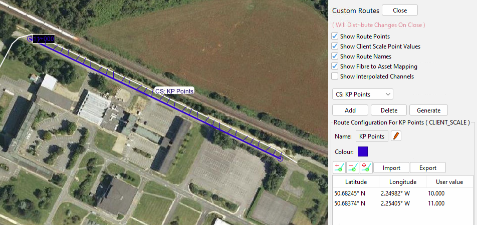
Figure 34: Client Scale with asset mapping enabled
Generating a Client Scale Using Customer Co-ordinates
In most cases, users would use the 'Add' button (Figure 33) to create a Client Scale and import customer-generated co-ordinated positions. However, in some cases, the resolution/accuracy of these co-ordinates may to too poor to follow the required Detector Route as intended. In this scenario, the 'Generate' option can be used that will generate a Client Scale that will fill any gaps with Detector Route coordinates between customer-generated coordinates.
To generate a Client Scale using Customer co-ordinates, press the 'Generate' button. This will open a dialogue in which the name, colour and parent Detector Route can be supplied. Ensure that the 'FromFile' tab is selected and that the customer CSV file has been selected. The OPSs this Client Scale should apply to also needs to be selected, and any spurs should be removed from consideration.
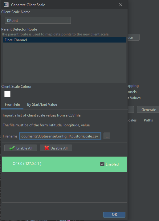
Figure 35: Generate the client scale using customer co-ordinates
When the OK button is pressed, a Client Scale will be created using a combination of customer and interpolated co-ordinates with a result similar to Figure 34.
A generated scale should be checked to ensure that it provides the expected mapping.
Markers
It is possible to add ‘Markers’ to the map display. An example of its use is having a marker represent a landmark like a security gate. To access the Markers section, select Markers from the Configure menu.
Figure 32 provides an overview of the Marker creation panel. To create a new marker type, select Add New Type. A new window will open, to which the user must give the marker type a name. Double click the default icon highlighted in red to open the icon selection window (Figure 38).
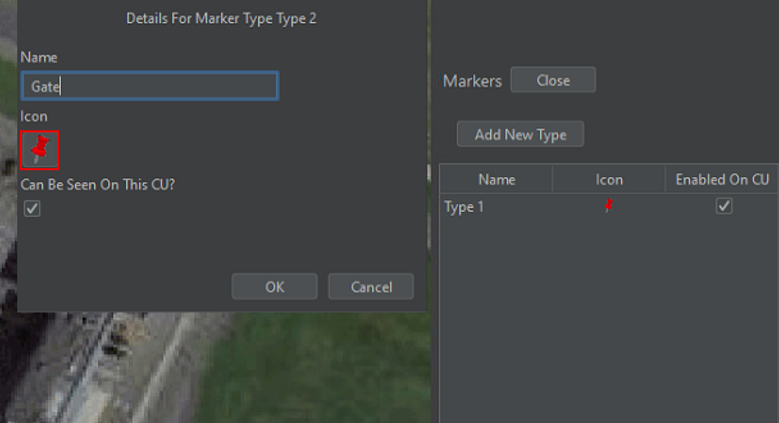
Figure 37: Creating New Marker
Select a different variation of the default marker or click the Load Custom Image to import your own image. Click Apply to add the new marker.
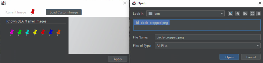
Figure 38: Creating New Marker Icon
Markers can then be added to the map display by opening the right-click menu at the required location and selecting Add Marker (Figure 39). Name the marker accordingly and select the required type from the Type drop-down menu. Checking the Priority box will give the marker priority over other markers being displayed at the same location.
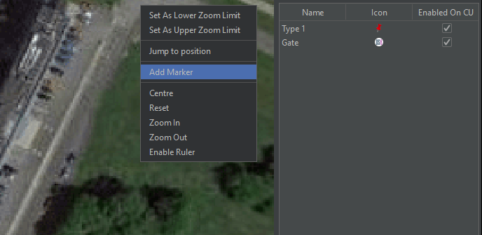
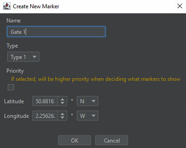
Figure 39: Creating New Marker Icon
Select OK (above image on the right) to add the marker to the map display (Figure 37).
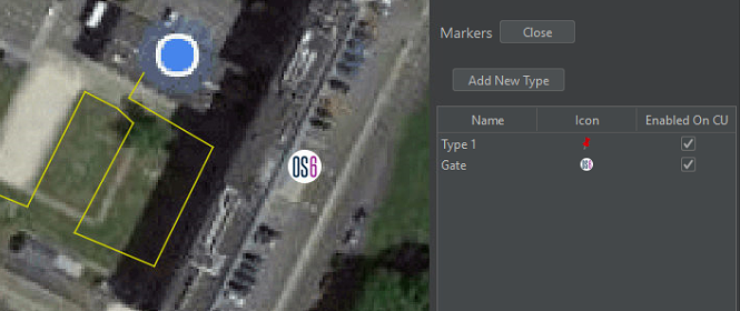
Figure 40: Icon Added to Map Display
Account Management
Account Management enables the creation of user accounts. Depending on the account setup, this will determine what role a user has on the system.
To access the Account Management section, select Account Management from the Configure menu.
In the Account Management window (Figure 41), select New User and fill out the subsequent window with the user details according to the type of user being set up. There are three accounts/roles to choose from.
-
Trained User - Includes Alert, Waterfall, Process and Limited Suppression Control + Many other configuration options.
-
User - Includes Alerts and Waterfall Controls + Limited Configuration.
-
Light User - Includes Alert and waterfall Viewing – Read Only.
Trained Users can be elevated to have full access over the system by checking the Can Login As Super-user box. Super-user access privileges require a time-sensitive One Time Passcode (OTP) that will need to be obtained from the OptaSense Authentication Server. The code will provide super-user access for 7 days before another code is required.
Once all the required information has been entered, select ok to add the user.
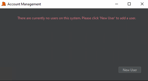

Figure 41: Left – Add New User / Right – Choose Role
Exporting Config
The current configuration can be exported by selected Export Config from the Configure>Config Management menu. In order to export a fully usable config, a validity check must be passed. However, the user can still proceed to export the system specification and maps for a config that has not passed the validity checks. This option can allow some parts of the config to be creator prior to a system install.
Check flags are available to specify whether to include the system specification and maps within the exported config.

Figure 42: Config Export panel
Press Next and then select the location to save the config and click Save to finish the export.
Additional Options
System
The System menu provides a means of exiting the software.
Display
The Display menu enables the user to toggle on / off certain visual layers currently displayed in the config.
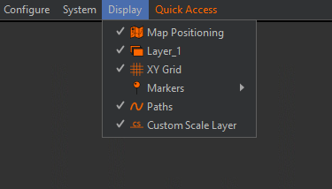
Figure 43: Display Section
Quick Access
The quick access section provides a list of recently used sections. Clicking on any of them will take the user to that section.
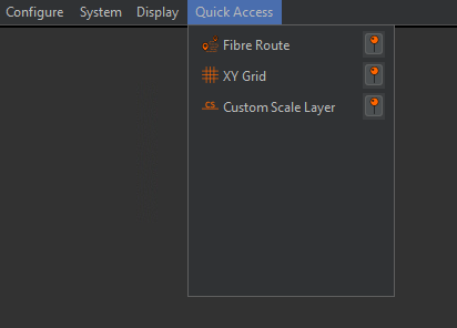
Figure 44: Quick Access